WOCE Indian Ocean Survey
Data Comparison at Crossover Stations
Analytical Procedure
The purpose of this analysis was to determine if any significant systematic offset existed between the various legs of the WOCE/JGOFS Indian Ocean survey of carbon measurements. Once the technique was developed, it was also applied to the salinity and silicate measurements from the same stations that were used for the carbon comparison. For reference and to obtain a general idea of the property distribution with depth, see Fig. 1, which shows both TCO2 and TALK distribution along longitude 90E (I8S + I9N).
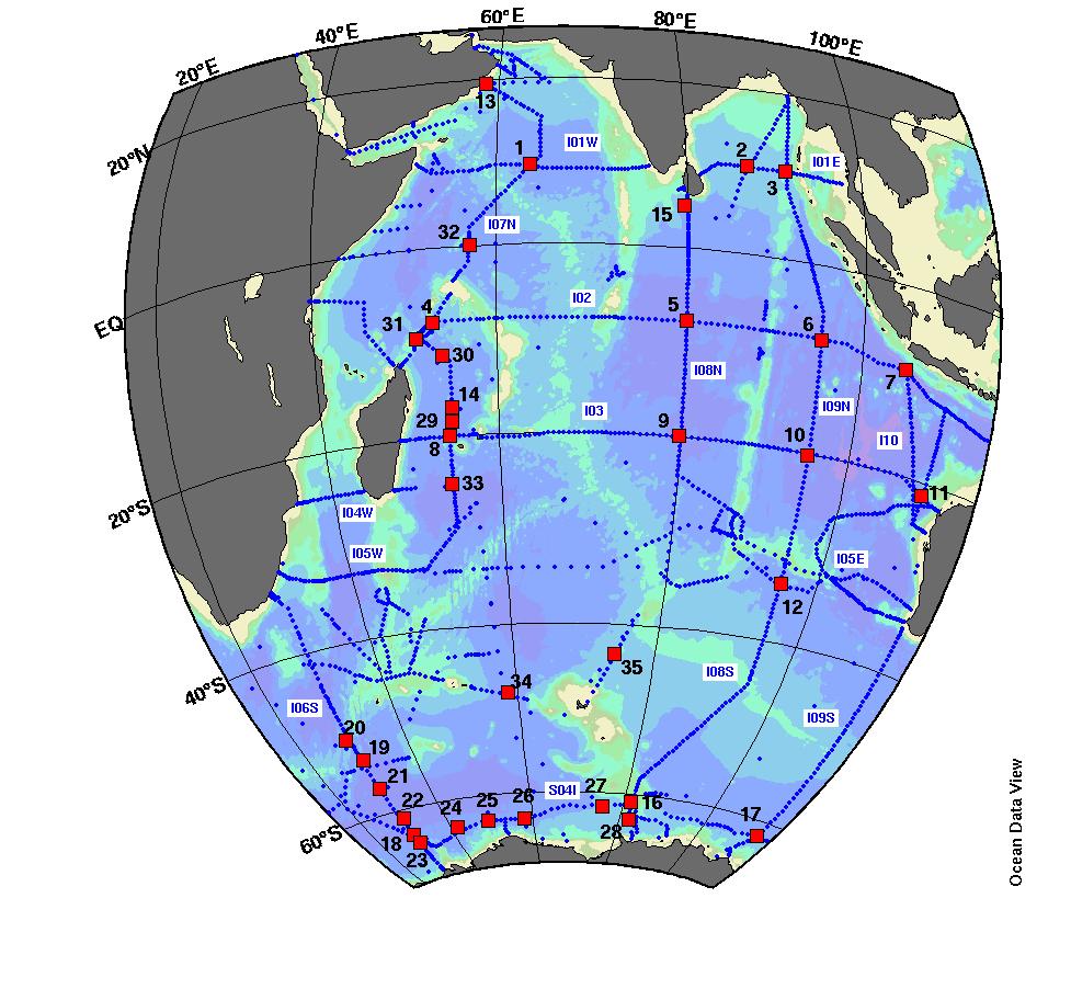
The stations selected for each crossover are those which are close to the crossover point and on which carbon measurements were made. Fig. 2 shows the locations of the 35 crossovers. The number of stations selected was somewhat subjective, but was such that sufficient measurements were present for the analysis without getting too far away from the crossover location. In all cases the stations were within approximately 1° of latitude or longitude of the crossover point. Table 1 lists the stations used for each crossover. Under the "Stations" column, numbers separated by a ":" imply an inclusive range of stations. In two cases the legs did not actually cross (crossover 7 and 14). The analysis here was done using the last station from one leg and the first from the next leg which had carbon data.
Once the stations were chosen, the data from the appropriate stations were plotted against potential density referenced to 3000 dB. Only data from pressures greater than 2500 dB was included. The data set used was the preliminary data prepared by either the SIO or WHOI CTD groups at the end of each leg. For each crossover a smooth curve was fitted to the combined station data from each leg so long as there were seven or more data points which could be used for the fit. The fitting curve chosen was a "robust loess" function designed to minimize the influence of outliers. In cases having less than seven points, linear segments were used to "connect the dots". Only data which had been marked with a quality control flag of 2 (good) or 6 (replicate) were included in the analyses and the salinity flags were applied to the calculated values.
In order to quantitatively estimate the mean difference between legs, each of the two fitted curves was evaluated at 50 evenly spaced intervals covering the range of space common to the selected stations from both legs. The 50 differences were then averaged. In each case the difference was taken as later cruise minus earlier cruise (or higher station number minus lower). Table 4 summarizes the mean differences and for all of the crossovers and indicates the sense of the differences in terms of the cruise leg designations (δ).
The data comparison plots for each crossover in Fig. 2 can be accessed from Table 4. Six plots were constructed for each crossover:
- Station Location - an expansion of the crossover area showing neighboring station locations (open symbols) and indicating which stations were used for the analysis (filled symbols).
- Data Summary - Full page plot with 6 small figures showing the data segregated by station.
- TCO2 Analysis - Detailed plot comparing total carbon dioxide with the data segregated first by cruise and then by station within each cruise. The line through the data for each leg is the fitted curve.
- Alkalinity Analysis - Detailed plot comparing total alkalinity with the data segregated first by cruise and then by station within each cruise. The line through the data for each leg is the fitted curve.
- Salinity Analysis - Detailed plot comparing salinity with the data segregated first by cruise and then by station within each cruise. The line through the data for each leg is the fitted curve.
- Silicate Analysis - Detailed plot comparing silicate with the data segregated first by cruise and then by station within each cruise. The line through the data for each leg is the fitted curve.
In addition to the individual crossover plots, four summary plots, one for each type of measurement, can be accessed via the last four column labels in Table 1.
In addition to the WOCE/JGOFS survey, NOAA carried out one cruise which repeated a portion of WOCE leg I8NI5E between 20°S and 5°N. For the overlap region, a somewhat more detailed comparison can be made. The data in the overlap region from each cruise were individually gridded as a section in vs space. The two gridded sections were then subtracted, the results contoured, and a mean difference calculated. This procedure was repeated for each of the four parameters used in the crossover comparisons. Only "good" data from pressures greater than 2500dB were used in the comparisons. These figures can be viewed using the links in Table 2.